(1) STATIC STRESS CHANGES

ΔCFF = Δτ + μ(Δσn + ΔP)

or ΔCFF = Δτ + μ’ Δσn

We can calculate static stress changes using software Coulomb [Link]

Assumption: computed in a homogeneous elastic half-space (Okada, 1992) [Link]

Some parameter need:

μ’ = 0.4  [possible value 0.0 -0.8] [Link] Strong fault: large μ (> 0.5). For example Sandstone, μ=06~0.8.

-Poisson ratio = 0.25

-Young’s modulus = 80 GPa

-Shear modulus = 32 GPa

Lower young modulus: Reduce magnitude of stress changes

Higher young modulus: Increase magnitude of stress changes

-Friction and Skempton coefficient not in substantial way providing variation.

-Shear and normal stresses produced by source can be resolved onto specific “receiver” fault or dyke.

-The receiver are defined by strike, dip and rake but Rake does not influence the normal stress changes!

Note:

Normal stress changes Δσn, positive if fault is unclamped

Shear stress changes Δτ, positive in the direction of fault slip.

We can calculated using published source fault models that I have compiled in here [Link].

Or you can use empirical fault geometry from Wells and Coppersmith (1994). [Link]

A new perspective on new paper: What Is Better Than Coulomb Failure Stress? A Ranking of Scalar Static Stress Triggering Mechanisms from 10^5 Mainshock-Aftershock Pairs (Meade et al., 2017) [Link]

 

(2) DYNAMIC STRESS CHANGES

σd = G. PGV / vs

where σd = radial peak dynamic stress; PGV = peak ground velocities; vs = shear wave velocity; G = shear modulus.

Shear modulus G can be derived from: G = ρ.vs^2 where ρ = rock density.

General value: G=35 GPa, vs=3.5 km/s

Rule of thumbs: 1 cm/s corresponds to ~ 0.1 MPa or 100 kPa.

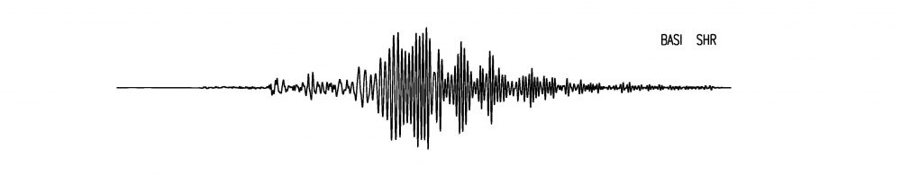
PGV are observed from seismogram!

Note: raw data from data center must be corrected with instrument response using pole and zero file.

Simply using transfer command in SAC. [see this tutorial].

Using command transfer to vel using BMKG waveform usually resulted in m/s (see the RESP file!)

How to get predicted PGV to calculate predicted dynamic stress?

(a) Using empirical relationship from magnitude

for near field (distance <= 500 km) using Campbell and Bozorgnia (2007)

log10 PGV = c1 + c2M – c3 log10 SQRT (r^2+c4^2)

where PGV in cm/s, M = magnitude, r = hypocentral distance (km), ci = fit parameters.

For unconstrained case, used c1=-2.29; c2=0.85; c3=1.29; c4=0.04.

For teleseismic field (distance > 500 km) using Lay and Wallace (1995) using Ms (surface wave magnitude) formula

log10 A20 = Ms – 1.66 log10 Δ – 2

A20= displacement in micrometers, Δ=distance in degrees

PGV ≈ 2πA20 / T

(Here we assume long-period surface wave with T = 20 seconds)

Both is available in van der Elst and Brodsky (2010) [Link]

Note: if using catalog with different magnitude type, convert to Ms using some empirical relationships. For example: Das et al. (2011) [Link] or Scordilis (2006) [Link]

(b) Using predicted PGV in shake map

Simply extract PGV data from shake map produced by some agencies such as USGS, or BMKG (in Indonesia).